Leafcutter Shiny App • leafcutter

Written by Jack Humphrey, David Knowles & Yang Li

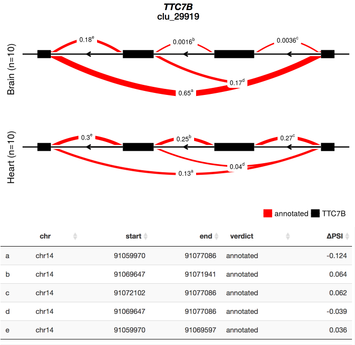
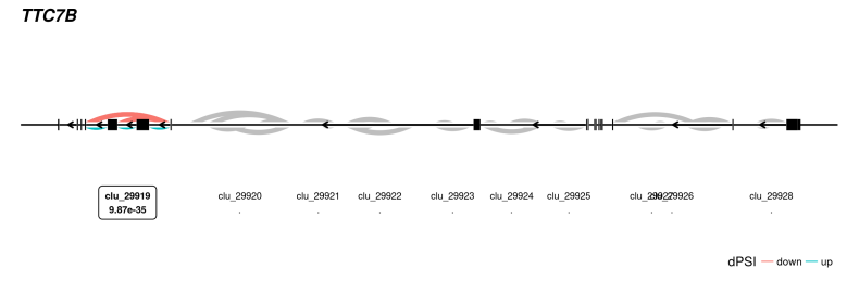
To see an example of the leafcutter shiny app in action without installing anything take a look at https://leafcutter.shinyapps.io/leafviz/. This shows leafcutter differential splicing results for a comparison of 10 brain vs. 10 heart samples (5 male, 5 female in each group) from GTEx.

The leafcutter shiny app has been tested on macOS 10.12 and Ubuntu 14.04.

Installation

UPDATE As of September 2020, LeafViz is now a standalone app. The original version of the app is still within the Leafcutter repository but will eventually be deprecated as all further maintenance and development will be to the standalone version.

## in R:
install.packages("remotes")
remotes::install_github("jackhump/leafviz")

## on the command line:
git clone https://github.com/jackhump/leafviz.git

Run Example

Once you’ve installed leafviz and downloaded the github repo then you can easily fire up a local shiny app on the same GTEx example data. Navigate into the leafviz directory:

cd leafviz/scripts

Now starting the shiny app should be as easy as

./run_leafviz.R example/Brain_vs_Heart_results.Rdata

You can even leave out the leafviz_example/Brain_vs_Heart_results.Rdata part as this is the default dataset run_leafviz.R will try to use.

Prerequisites: Annotation data

The Shiny app includes functionality to label detected introns as annotated or cryptic. To do for a new dataset this an “annotation code” is needed, built from a “Gene Transfer Format” file appropriate for your genome. We provide pre-built annotation codes for hg19 and hg38 which can be downloaded by running

./download_human_annotation_codes.sh

from the leafviz directory. To build a new annotation code requires perl.

This step processes a given GTF to generate lists of exons, introns and splice sites. This step only has to be run once to use a particular GTF file with the app.

The recommended way to do this is

./gtf2leafcutter.pl -o <annotation_code> my_transcriptome.gtf[.gz]

my_transcriptome.gtf - a gene transfer format file, provided by GENCODE, Ensembl, etc.

annotation_code - the path or folder name with a base name, eg /path/to/gencode_hg38

gtf2leafcutter.pl can take in a gzipped gtf file as long as the file name ends with .gz.

(thanks to Dalila Pinto for contributing the new script).

This will create:

<annotation_code>_all_introns.bed.gz
<annotation_code>_threeprime.bed.gz
<annotation_code>_fiveprime.bed.gz
<annotation_code>_all_exons.txt.gz

We’ve only tested with the GENCODE human GRCh37/GRCh38 and mouse GTF files. If you have problems with other gtf files please let us know.

Step 1. Prepare the LeafCutter differential splicing results for visualisation

This step annotates each intron in each cluster at a given false discovery rate and generates a single .RData file with everything the shiny app needs to run.

leafcutter/leafviz/prepare_results.R [options] <name>_perind_numers.counts.gz <name>_cluster_significance.txt <name>_effect_sizes.txt annotation_code

** _perind_numers.counts.gz ** The same counts matrix you gave to leafcutter_ds.R. ** _cluster_significance.txt ** The cluster significant table output by leafcutter_ds.R. ** _effect_sizes.txt ** The per junction effect size table output by leafcutter_ds.R. ** annotation_code ** will be something like annotation_codes/gencode_hg19/gencode_hg19 (see above)

Options:

    -o OUTPUT, --output=OUTPUT
        The output file that will be created ready for loading by run_leafviz.R [leafviz.RData]

    -m META_DATA_FILE, --meta_data_file=META_DATA_FILE
        The support file used in the differential splicing analysis. Columns should be file name and condition

    -f FDR, --FDR=FDR
        the adjusted p value threshold to use [0.05]

    -c CODE, --code=CODE
        A name for this analysis (will be available in leafviz through the Summary tab). [leafcutter_ds]

    -h, --help
        Show this help message and exit

This will create the Rdata file wherever --output is pointed. The file ‘prepare_example.sh’ shows how this would be done for the example dataset if you wanted to rebuild ‘Brain_vs_Heart_results.Rdata’.

As a concrete example, let’s assume you just ran the example at Usage and you’re within the leafcutter/ top directory .

cd leafviz/
./prepare_results.R --meta_data_file ../example_data/example_geuvadis/groups_file.txt \
  --code leafcutter ../example_data/testYRIvsEU_perind_numers.counts.gz \
  ../example_data/leafcutter_ds_cluster_significance.txt \
  ../example_data/leafcutter_ds_effect_sizes.txt \
  annotation_codes/gencode_hg19/gencode_hg19 \
  -o testYRIvsEU.RData

should create an testYRIvsEU.RData file.

Step 2. Visualise the results

From the example_data directory.

cd <leafviz repo>/scripts/
./run_leafviz.R testYRIvsEU.RData

This will load in the Rdata object and run the LeafCutter Visualisation App in your browser.

Features

Visualisation of significantly changed clusters

cluster plot example

Visualisation of all clusters discovered in a gene

gene plot example

PCA plot based on splice junction counts
All plots can be exported as PDF